CROP EXPLORER
Crop Modeling Platform
Implemented crop models: AquaCrop · WOFOST · APSIM Next Generation · DSSAT (experimental wheat)
Illustrated user manual · Working draft 0.8 | 27 October 2026
Center for Applied Systems Analysis, College of Agriculture and Environmental Sciences (CAES), University Mohammed VI Polytechnic (UM6P)
CROP EXPLORER
Implemented crop models: AquaCrop · WOFOST · APSIM Next Generation · DSSAT (experimental wheat)
Illustrated user manual
Center for Applied Systems Analysis, College of Agriculture and Environmental Sciences (CAES), University Mohammed VI Polytechnic (UM6P)
Working draft 0.8 | 27 October 2026
Purpose
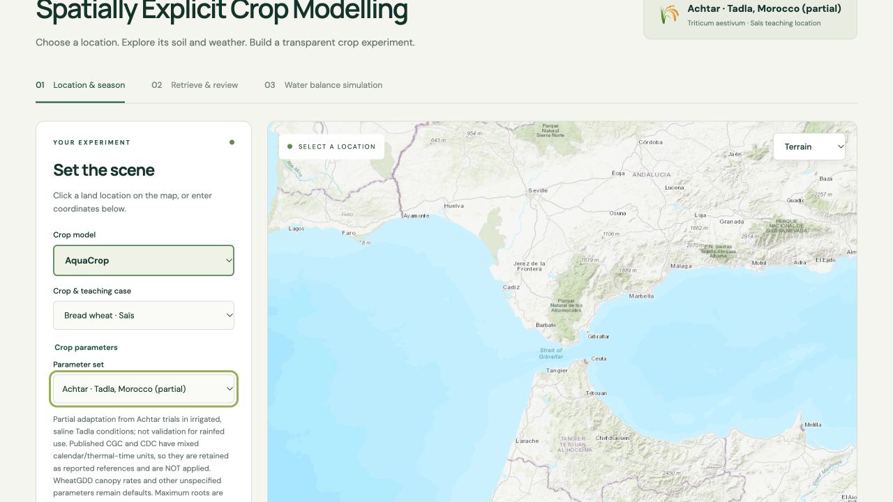
Use CropExplorer to explore environmental inputs and build transparent rainfed cereal simulations for teaching. This guide follows the current local interface and uses saved AquaCrop teaching-run figures to illustrate outputs.
Read results as experiments. Model defaults, partial published adaptations and gridded inputs do not by themselves establish a locally validated field forecast. Numerical water-balance closure checks conservation, not agronomic accuracy.
In this draft: Background & model comparison | 1 Start & select | 2 Retrieve & review | 3 Soil water | 4 Simulate | 5 Interpret & export | 6 Sadoré | 7-10 New features | 11-15 Moroccan parameters | 16 Saïs comparisons | 17 High Atlas barley | 18 Four-model wheat comparison
Background / How crop modeling works
A model is a structured experiment
A crop model represents how a crop develops and grows in response to weather, soil, crop traits and management. It turns explicit inputs and assumptions into a time series of crop and soil conditions. A simulation answers a conditional question: what could happen under this scenario? Its usefulness depends on whether the represented processes and input data suit the question. [1, 2, 5]
Three broad approaches
Empirical and statistical models learn relationships between observations, such as yield and seasonal weather. They can support prediction where representative training data exist; extrapolation to unfamiliar climates or management requires care. Process-based models describe development, growth and resource balances through biological and physical relationships. Hybrid approaches combine process descriptions with statistical learning or observations. These are broad categories; individual tools often mix methods.
The daily soil-crop-weather loop
- Read weather and management: temperature, radiation, rainfall and any scheduled operations.
- Advance phenology: emergence, flowering and maturity depend on the crop and its development parameters.
- Update canopy or leaf area, intercepted radiation, transpiration and biomass production.
- Update soil water and, where represented, nutrients; calculate how shortages or excesses affect crop processes.
- Allocate growth among organs and update roots, biomass, grain and the conditions for the next day.
This sequence is a teaching summary. Equations, ordering and feedbacks differ among models. AquaCrop links biomass to transpiration; WOFOST calculates assimilation from absorbed light and subtracts respiration. [1, 2]
Inputs, parameters, states and outputs
Inputs drive a scenario: daily weather and management. Parameters describe properties such as development requirements and soil retention. States carry memory, including soil water, leaf area and biomass. Outputs are selected states and fluxes, such as yield, evapotranspiration, runoff and drainage. Initial states matter: two identical seasons can differ when starting soil water differs.
Background / Major established model families
The following selection covers widely used crop and farming-system tools. It is an orientation, rather than an exhaustive list or a ranking. Capabilities vary by crop module, release and configuration. CropExplorer now exposes AquaCrop, WOFOST, APSIM Next Generation and experimental DSSAT CERES-Wheat. DSSAT currently runs the Newton IB0488 wheat reference; crop availability and server configuration differ.
| Model / family | Main emphasis | Typical questions |
| AquaCrop [1] | Water-driven crop growth; canopy cover, transpiration, biomass and harvest index. | How does water availability or irrigation affect crop production? |
| WOFOST [2] | Daily crop development, photosynthesis, respiration and biomass partitioning. | What are potential and water-limited production and seasonal crop development? |
| DSSAT [3] | A suite of crop models, including CERES and CROPGRO, with soil-plant-atmosphere interactions. | How do cultivar, planting, water and nutrient management affect crop outcomes? |
| APSIM [4] | A modular farming-systems framework coupling crop, soil and management models. | How do management rules and sequences of crops affect system performance? |
| STICS [5] | Daily soil-crop functioning with energy, water, carbon and nitrogen balances. | How do crop sequences, irrigation and nitrogen management affect production and losses? |
| EPIC / APEX [6] | Agricultural production, hydrology and soil/land management; applications from fields to larger spatial systems. | How do land-management and climate scenarios affect production and environmental outcomes? |
Choose for the question and the evidence
For a water-productivity lesson, AquaCrop provides a direct connection between water use and biomass. For an explanation of radiation-driven crop growth, WOFOST offers a contrasting approach. Questions about rotations, nutrient cycling or environmental losses may require a broader framework and additional data. Greater process detail also creates more parameter and evaluation requirements.
A model family is not an implementation
CropExplorer uses AquaCrop-OSPy, WOFOST 7.2 through PCSE, APSIM Next Generation and an experimental DSSAT CERES-Wheat adapter, each with specific settings. Features described for the wider model families are not automatically available here. For example, CropExplorer currently runs rainfed scenarios, and its WOFOST soil configuration is homogeneous over the selected depth.
Background / Interpretation and model evaluation
Potential, limited and actual production
Potential production describes growth under the specified weather and crop characteristics when water and nutrients do not limit it. Water-limited production includes the effect of soil-water availability. Actual farm yield can also reflect nutrient shortages, pests, diseases, weeds and management constraints. A simulated water-limited yield should not automatically be interpreted as actual farm yield. These distinctions are central to WOFOST production analysis. [2]
Calibration is different from evaluation
Calibration adjusts defensible parameters to observations, such as flowering dates, leaf area, soil moisture, biomass and yield. Independent evaluation tests the resulting configuration against observations not used to tune it, ideally across seasons and sites relevant to the intended use. Matching one yield value can hide errors in timing, water use or biomass allocation.
Four sources of uncertainty
Input uncertainty: weather grids, estimated hydraulic properties and missing days. Parameter uncertainty: cultivar development, rooting and stress-response values. Structural uncertainty: the processes included, omitted or simplified. Scenario uncertainty: future weather and management choices. Comparing models explores some structural differences, but model agreement alone does not establish correctness.
What this means in CropExplorer
The map locates an input sample; it does not make a point simulation a spatially distributed field model. Model defaults are teaching starting points; published partial Moroccan profiles can now be selected, with their limitations retained. APSIM and DSSAT now include nitrogen dynamics and stress; AquaCrop and WOFOST omit nutrient limitations in the current configurations. Several constraints affecting actual yield remain omitted, and the High Atlas case requires particular care with snow, freezing and elevation gradients. Keep these boundaries with every exported interpretation.
A passing balance is one check
Water-balance closure tests whether accounted inputs, outputs and storage changes conserve water numerically. It does not demonstrate that rainfall, soil properties, stress responses or yield match the real field. Combine numerical checks with observed-data evaluation and sensitivity analysis.
A useful comparison exercise
Run compatible engines with the same location, crop, weather window and comparable initial conditions. Compare maturity, actual ET, biomass and yield. Record model-specific parameters and soil representations. Then change rooting depth or initial water in each model. Explain differences through assumptions and processes before deciding which result better fits observations.
Background / CropExplorer model strengths and best fit
This guide compares the four engines as currently configured in CropExplorer. The strengths and limits below describe these adapters, not every capability of each model family. “Best fit” means a good match for a teaching or analysis question; it is not an accuracy ranking.
| Model | Strengths in CropExplorer | Current limitations | Best fit for |
| AquaCrop [1, 13] | Clear water-productivity framework links canopy, transpiration, biomass and grain; layered soil-water views are available. | Nutrient limitations are omitted. Crop defaults and partial transfers need local evaluation. Current scenarios are rainfed. | Rainfed water-productivity lessons and sensitivity to rainfall, starting water, roots and soil layers. |
| WOFOST [2, 14] | Useful daily view of crop development, radiation-driven growth, biomass and leaf-area index (LAI); water-limited runs can stop at maturity. | Soil properties are averaged into one homogeneous profile over selected depth. Nutrient stress is omitted; radiation, humidity and wind inputs are required. | Seasonal phenology, LAI and biomass, or water-limited scenarios for supported wheat, barley, maize and millet templates. |
| APSIM Next Generation [4, 15] | Coupled crop and soil processes, layered water, and active nitrogen dynamics/stress for supported wheat, barley and maize examples. | Needs complete soil and weather inputs. Adapter soil/nitrogen settings are assumptions; local cultivar calibration, P/K stress, pests and diseases are not provided. | Supported crop-management questions where nitrogen effects and layer-specific soil-water processes matter. |
| DSSAT CERES-Wheat [3, 26, 27] | Experimental wheat runs include water and nitrogen stress, daily LAI, root-depth and six-layer moisture outputs, and the reference Newton IB0488 cultivar. | Experimental wheat-only pathway; Newton IB0488 is not locally calibrated. Selected depth guides root distribution but does not cap root-tip depth. Crop workbooks are not supported. | Technical pilot, explicit fertilizer scenarios, or side-by-side reference-wheat comparisons. Not yet for other DSSAT crops or local yield recommendations. |
How to choose: Select the engine whose represented processes match the question, then keep cultivar, soil representation, management and calibration status attached to the result. A more detailed process model is not automatically more accurate; validate against independent local observations.
1 / Start and select your experiment
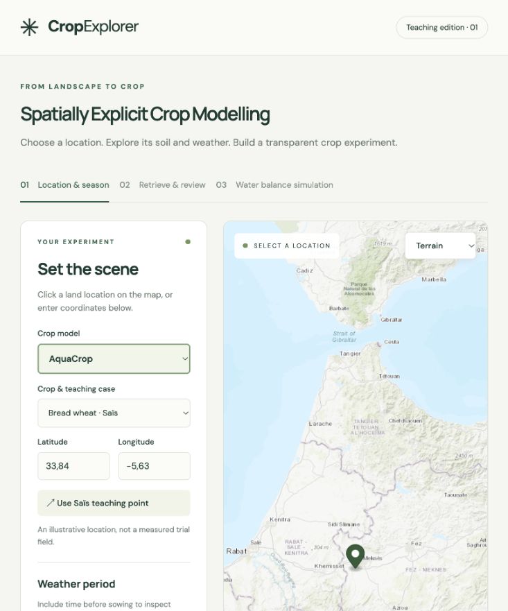
Open CropExplorer
On the configured Mac, double-click Start CropExplorer.command, then open http://127.0.0.1:8010. If an instance is already running, use it. Retrieval requires a working Google Earth Engine connection; the configuration indicator is not proof that a retrieval will succeed.
- Choose Crop model: AquaCrop, WOFOST, APSIM Next Generation or experimental DSSAT CERES-Wheat (where configured). Keep this choice and the selected crop parameter profile with your experiment notes.
- Choose Crop & teaching case: Bread wheat · Saïs, Barley · High Atlas, Pearl millet · Sadoré, Niger, or Tropical maize · Katumani, Kenya. Teaching points are illustrative locations, not measured trial fields.
- Click a land location on the map, or enter latitude and longitude. Use negative longitude west of Greenwich. The Saïs example is 33.84, -5.63; the High Atlas example is 31.65, -6.43.
- Set the Weather period. Both endpoints are included; retrieval accepts up to 1,461 daily records. Each simulation is one season of at most 300 days. Include the intended simulation season and, where useful, time before sowing to inspect conditions.
- Choose Terrain, Satellite or Hybrid to inspect the point. A basemap helps locate a site; it does not establish field boundaries or soil representativeness.
A first teaching exercise
Start with AquaCrop and Bread wheat · Saïs, with weather from 1 September 2023 to 31 July 2024. Later compare scenarios by changing one assumption at a time and saving each complete record.
What is sampled?
ERA5-Land: daily reanalysis weather at approximately 11 km resolution.
SoilGrids: estimated soil properties for six intervals between 0 and 200 cm, sampled at approximately 250 m. [17]
HiHydroSoil: estimated hydraulic properties derived from soil information, rather than direct field measurements.
2 / Retrieve and review inputs
- Click Retrieve soil & weather and keep the page open while retrieval is running.
- Read the status message and summary metrics. In Daily weather, compare rainfall with reference evapotranspiration (ET0). Monthly bars sum valid daily records; partial months and missing days need attention.
- Open Inspect the daily weather table when a period looks unusual. Missing or invalid days are excluded from the retrieved weather; they are not automatically filled.
- Open Sources & quality. Review coverage, warnings and assumptions before moving to simulation.
- Open Soil profile and inspect depth patterns, gaps and hydraulic validity. Complete values alone do not establish that the estimates represent the field.
If you change the selection
Changing location, crop or dates can make the displayed results stale. Retrieve again. Existing input downloads retain the original retrieved location and dates; check the full record before combining files.
Reading ET0
ET0 expresses atmospheric evaporative demand for a reference surface. It is not simulated crop water use. CropExplorer calculates it with FAO-56 Penman-Monteith assumptions; daily mean wind components can underestimate mean wind speed and ET0.
When retrieval fails
Check that the local server remains running and inspect the connection/status message. Confirm the configured Earth Engine project and access through the installation administrator. Retry the same selection. If a source is missing, inspect its warning rather than treating blank values as zero. Hydraulic retrieval failure may leave weather and other soil inputs available.
Capture status for this draft
The original interface capture and saved AquaCrop teaching figures are retained as historical illustrations. Chapters 16-17 include fresh captured charts from current Saïs comparison runs and a live High Atlas WOFOST barley run; Chapter 18 adds the four-engine wheat comparison. These are teaching scenarios, not field validation.
3 / Review soil and hydraulic properties
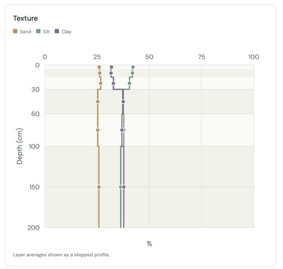
Read profiles by depth
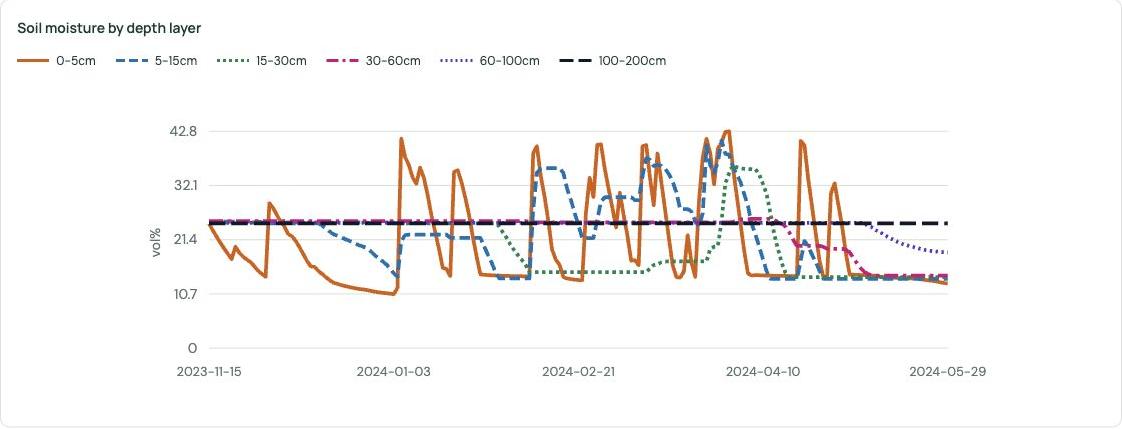
The six intervals are 0-5, 5-15, 15-30, 30-60, 60-100 and 100-200 cm. Texture and coarse fragments are percentages; organic carbon is g/kg and bulk density is g/cm3. Gaps indicate missing or out-of-range values. Hover over chart points in the platform for individual layer values.
Review water retention and conductivity
WP is wilting point, FC is field capacity and SAT is saturation, expressed as volumetric water percentages. Ksat is saturated hydraulic conductivity in mm/day. Valid ordering is WP < FC < SAT, with positive Ksat. The default FC estimate uses pF 2 (about -10 kPa); review whether that definition suits the soil. [18]
Use measured replacements carefully
Edit hydraulic cells only when you have defensible values. Confirm the FC definition and enter a source note, such as a laboratory report and method. Edits are labelled User supplied and apply to the session and downloads. Restore retrieved estimates returns the original estimates. Save the full input record to retain provenance.
4 / Configure and run a simulation
- Scroll to the model water-balance section after retrieving inputs. Review the crop/model description and expand Review model assumptions.
- Set the sowing/initial-water date and latest simulation date within the available weather period. The actual run may finish earlier.
- Set maximum rooting depth and initial available water. In this interface, 0% initial available water means WP and 100% means FC; this is not the same as volumetric moisture percentage.
- For AquaCrop and APSIM, review their curve-number settings. For WOFOST, review the non-infiltrating rainfall fraction. These controls represent different model assumptions and should not be equated. For APSIM and DSSAT, review planting, nitrogen and soil settings; DSSAT interprets selected depth as a root-distribution setting, not a hard root-tip limit (Chapter 18).
- Leave gap interpolation off unless you explicitly accept its assumptions. Opting in permits linear interpolation of interior gaps of one or two days, including rainfall. Inspect and save every filled value.
- Click the run button, then inspect the status, stopping reason, simulated dates and numerical water-balance check before reading yield.
Choose the model with its assumptions in mind
AquaCrop: AquaCrop-OSPy 3.1.0. The soil is represented with layers and compartments. With Model default, wheat uses calendar-day phenology and barley uses thermal time; selected partial profiles can change that basis. Layer moisture curves are available.
WOFOST: WOFOST 7.2 water-limited production through PCSE 6.0.13. This configuration averages soil properties over the selected maximum root/profile depth. It reports leaf-area index (LAI); separate six-layer moisture curves are unavailable. It also needs radiation, humidity and wind, so older input records may need retrieval again.
High Atlas barley
The illustrative case uses a point near Tabant and editable February sowing assumptions. Inspect whether maturity was reached. Snow accumulation/melt, freezing, terrace hydrology and local vernalization are not explicitly represented. Coarse weather grids cannot resolve field elevation gradients. Teaching defaults are not local sowing recommendations.
5 / Interpret, save and compare
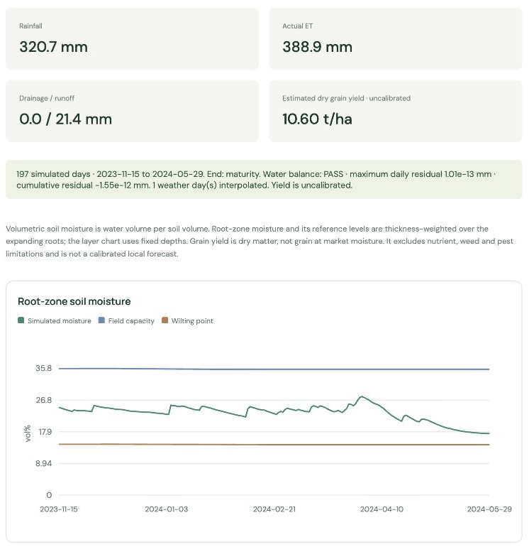
Read the result in this order
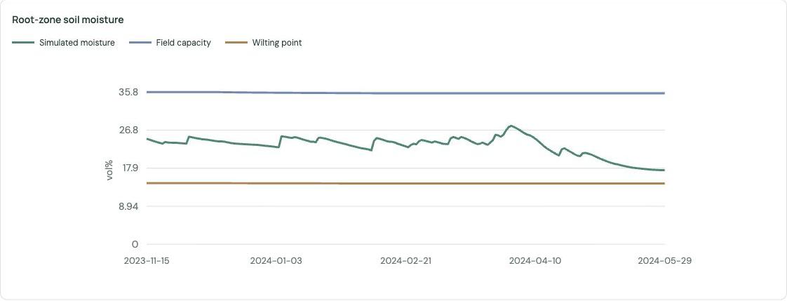
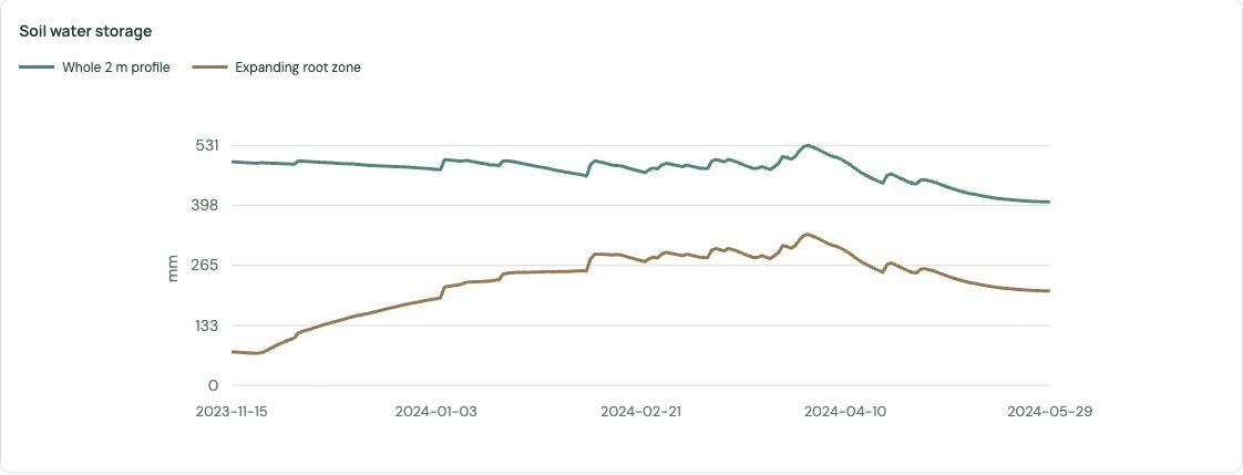
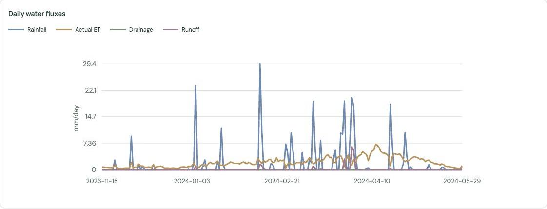
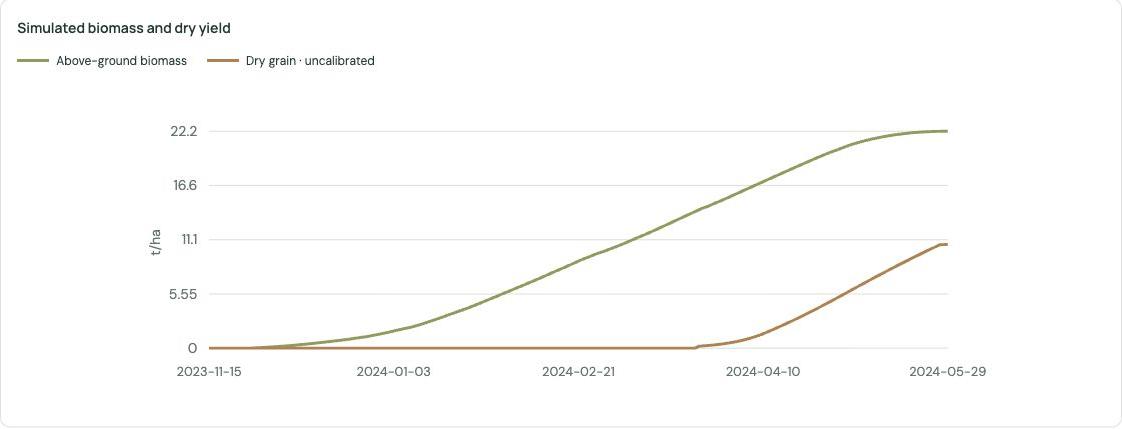
First: check dates, maturity/stopping reason, warnings and water-balance status. Next: compare rainfall, actual ET, runoff and drainage. Then: inspect moisture against FC and WP. Root-zone averages change as roots expand; fixed-depth curves answer a different question. Finally: consider dry grain yield and biomass, with model limitations in view. Dry grain yield is not adjusted to commercial moisture content.
Keep a reproducible experiment
Save Weather CSV, Soil CSV, Hydraulics CSV and the Full input record. After simulation, optionally export the Illustrated Excel report (.xlsx) and save Daily simulation CSV and the Complete simulation record. Keep scenario assumptions and any gap filling with the results. Compare one changed assumption at a time.
About this draft
Based on the local interface, application source and project notes on 27 October 2026. Figure 1 was captured for edition 0.1; Figures 2-3 are cropped existing project images; Figure 4 is a saved Sadoré integration capture. Figures 6-15 document the earlier Saïs comparison; Figures 16-20 are fresh live High Atlas screen captures; Chapter 18 compares four wheat-model outputs from the 27 October 2026 loaded-input view. Chapters 7-15 document platform additions and Moroccan parameter evidence. Source images and run records are retained in output/pdf/figures.
6 / Sadoré: pearl millet in Niger
Why this case?
The Sadoré example connects a published crop-modeling study with an exploratory platform experiment. Use it to distinguish experimental observations, published calibration references and assumptions introduced when changing model or weather source.
The published study
Akponikpè, Gérard, Michels and Bielders (2010) used APSIM to study pearl millet and nitrogen management in the Sahel. Field experiments at the ICRISAT Sahelian Centre combined manure, millet residues and mineral fertilizer during contrasting 1994 and 1995 seasons. The study also examined management over 23 years of weather. Its central question concerned production and risk under variable rainfall and fertility. [7]
The CropExplorer teaching configuration
Select Pearl millet · Sadoré, Niger. The case sets the point to 13.25 N, 2.283333 E and the initial retrieval window to 1 May-31 October 1994. WOFOST is selected automatically; AquaCrop, APSIM and DSSAT are unavailable for this crop. The runnable crop template is Millet_VanHeemst_1988, not a calibrated CIVT cultivar.
A research reference, an executable experiment
The published cultivar is CIVT (Composite Inter-Varietal de Tarna). The platform retains experimental metadata and downloadable APSIM parameter references, while running generic WOFOST pearl millet. APSIM thermal sums, radiation-use efficiency and soil drainage coefficients have not been substituted into WOFOST coefficients. CropExplorer does not simulate the nitrogen and phosphorus treatment responses of the source study.
Keep the seasons separate
The local reference record reports sowing on 6 June 1994 with a final stand of 25,000 plants/ha, and on 20 June 1995 with 30,000 plants/ha. Reported harvest dates are 20/23 September 1994 and 26/27 September 1995. These are experimental metadata, not all active controls in the current model. The approximate 95-day cultivar description is not an observed harvest date or a guaranteed WOFOST duration.
What the default assumptions mean
Maximum roots of 1.5 m and 50% initial available water are editable assumptions. The screenshot uses a latest simulation date of 23 October 1994, a model window limit rather than the experimental harvest date. ERA5-Land supplies weather; it is not the station weather used to document the field experiment. A run with these settings explores a scenario and does not reproduce the published APSIM experiment.
Teaching comparison
Compare retrieved and published water limits with other inputs fixed. Interpret storage and stress changes; this does not validate CIVT yield or fertilizer response.
6 continued / Run and document the Sadoré case
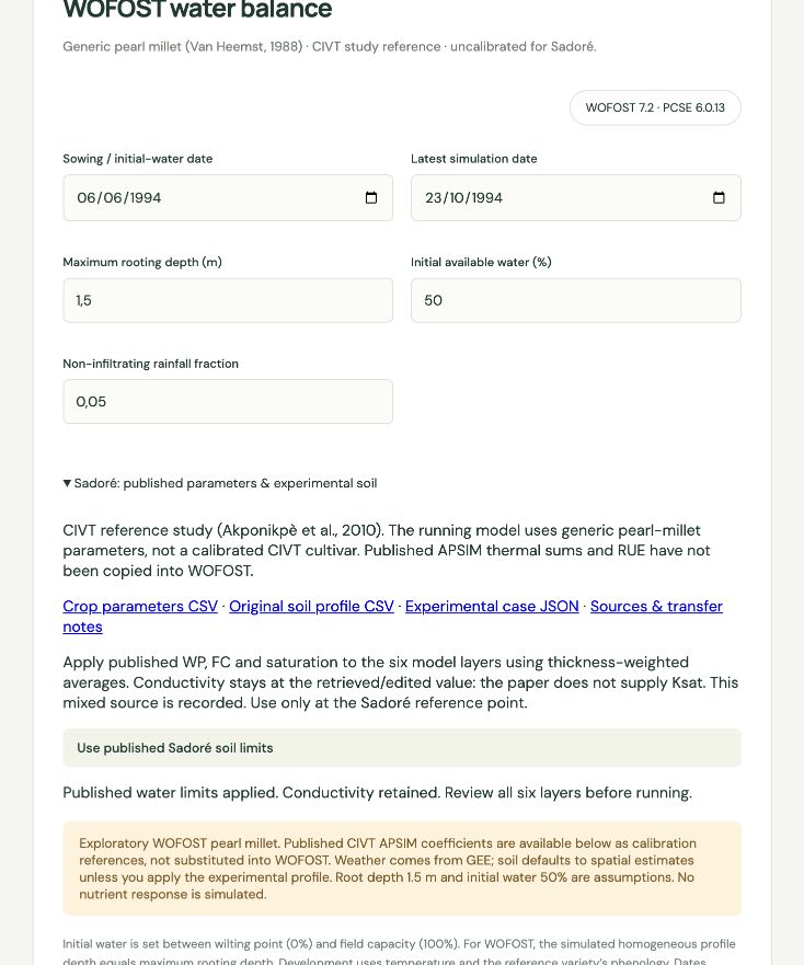
- Select the Sadoré case and retrieve inputs at its teaching point. Review weather coverage and the soil profile. After retrieval, check the suggested sowing date of 6 June 1994 and the latest simulation date.
- Expand Sadoré: published parameters & experimental soil. Download the crop-parameter CSV, original soil-profile CSV, experimental-case JSON and transfer notes to preserve the research context.
- To explore the experimental water limits, click Use published Sadoré soil limits. The control requires current retrieved inputs at the Sadoré reference point. Review the resulting six layers before running.
What the soil control changes
It maps the original nine-layer LL15, DUL and SAT values into the six standard horizons using thickness-weighted averages, and uses them as WP, FC and saturation. DUL was calibrated in APSIM and SAT was calculated. Ksat retains the retrieved or edited value; texture remains SoilGrids. This mixed-source profile is recorded. The crop extraction lower limit of 0.044 is distinct from soil LL15. WOFOST subsequently averages the soil over the selected depth.
- Review roots, initial water and the non-infiltrating rainfall fraction, then run. Inspect dates, maturity/stopping reason, balance status, LAI, actual ET and biomass before interpreting grain yield. Save the full input and simulation records.
7 / Current capabilities and new workflow
Edition 0.8 | 27 October 2026
This edition adds a model-selection guide comparing strengths, limits and best-fit questions, and documents DSSAT CERES-Wheat as a fourth, experimental engine alongside crop-parameter selection, Kenyan maize, illustrated Excel reports, longer weather retrieval and source traceability. The earlier figures remain labelled historical teaching captures. Screenshots illustrate interface states; they do not establish validation of the underlying scenario.
| Crop / case | AquaCrop | WOFOST | APSIM Next Generation | DSSAT CERES-Wheat |
| Wheat · Saïs | Default + partial Achtar | Default + 8 Moroccan timing profiles | Hartog reference | Newton IB0488 reference |
| Barley · High Atlas | Default + shared Egyptian-trial reference | Spring_barley_301 default | Dash reference | Unavailable |
| Tropical maize · Katumani | Maize default | Maize_VanHeemst_1988 | Dekalb_XL82 reference | Unavailable |
| Pearl millet · Sadoré | Unavailable | Millet_VanHeemst_1988 | Unavailable | Unavailable |
Select the crop, engine and parameter set
Under Crop parameters, choose Parameter set. Model default remains available. Read Sources & availability for the selected combination and download the catalogue or transfer notes. Disabled research entries identify evidence that has not been converted into an executable profile. A profile changes crop parameters; it does not move the map point or replace weather, soil or management.
Longer weather history, one season per run
Retrieve up to 1,461 daily records, equivalent to four years including a leap day. Weather tables and input downloads retain that complete request. A simulation still represents one selected season, at most 300 days; only weather within its run window is used. Repeated seasons require separate scenario runs, not a multi-year crop rotation in this interface.
Keep a complete scenario record
Record crop, model, profile, dates, initial water, rooting depth and engine-specific settings before comparison. Full simulation exports preserve profile identifiers, applied overrides, source notes, omitted values, soil transformations and weather adjustments. Download the complete JSON for the detailed audit trail.
Platform author
Bruno Gérard
Center for Applied Systems Analysis · College of Agriculture and Environmental Sciences · University Mohammed VI Polytechnic (UM6P).
8 / APSIM Next Generation
What is now implemented
The platform server runs APSIM Next Generation with SoilWater + Nutrient + PMF for wheat, barley and maize. Students do not need a local APSIM installation. The operator must provide a licensed/configured installation and its example files. The exact engine version and source information are retained in the complete run record. [4, 15]
Reference cultivars and inputs
The running reference cultivars are Hartog wheat, Dash barley and Dekalb_XL82 maize. None is a Moroccan cultivar calibration. APSIM needs site information, radiation, humidity, wind, hydraulic limits, bulk density and organic carbon for all six horizons. If these are missing, retrieve complete inputs again.
| Scenario setting | Current cereal default | Interpretation |
| Population; sowing depth; row spacing | 120 plants/m2; 30 mm; 250 mm | Editable management assumptions |
| Initial nitrate-N; ammonium-N | 60; 5 kg/ha | Whole-profile totals distributed by layer thickness over 2 m |
| Nitrate-N at sowing | 100 kg/ha | Single application; not a local recommendation |
| Constant CO2 | 400 ppm | Explicit scenario value, not historical reconstruction |
Review nitrogen and soil assumptions
APSIM and DSSAT include nitrogen dynamics and stress; AquaCrop and WOFOST omit nutrient limitations in these configurations. The adapter assumes pH 7, C:N 12, microbial fraction 0.02, inert fraction 0.6 and no initial residues. Soil carbon from g/kg is converted to percent. Crop extraction LL equals WP; KL is 0.06/day above the root limit, and deeper root exploration is blocked. SWCON is 0.3/day; evaporation U and CONA are both 5. These are adapter assumptions, not measured site parameters.
Saturation and porosity
If saturation exceeds porosity calculated from bulk density, the run stops by default. The optional checkbox caps saturation using particle density 2.65 g/cm3 and records each change. It does not alter the retrieved record or validate either estimate. FC at or above that porosity still requires input review.
Read outputs with the engine conventions
APSIM computes potential evaporation internally; retrieved ET0 is a comparison value. Results use end-of-day states, include interception evaporation in actual ET and report LAI. The run has one sowing and no automatic harvest/resowing; inspect harvest readiness and the end date. Rainfed configuration, phosphorus stress, pests and weeds remain outside the configured scope.
9 / Katumani: tropical maize in Kenya
A comparison case, not a cultivar trial
Choose Tropical maize · Katumani, Kenya. The illustrative point is 1.58 S, 37.24 E. The case uses March-September 2024 weather, 15 March sowing, 1.2 m maximum roots and 50% initial available water. These are editable teaching assumptions. The point is not a measured trial field; KALRO provides agronomic context, not a calibration for these engine parameter sets. [20]
OPV and Hybrid labels
Select open-pollinated variety (OPV) or Hybrid to record the scenario type. Within each engine both choices currently use the same parameters. The app does not simulate a genetic advantage for Hybrid. A change in this label alone should not be interpreted as a crop-genetic experiment.
| Engine | Reference parameter set | Yield and interpretation |
| AquaCrop | Maize; 132-day calendar cycle | Dry grain; nutrient stress omitted |
| WOFOST | Maize_VanHeemst_1988 | Whole cob dry matter, not shelled grain; nutrient stress omitted |
| APSIM Next Generation | Dekalb_XL82 | Dry grain with nitrogen dynamics; 6 plants/m2 and 750 mm rows as maize defaults |
Do not compare unlike yield definitions
WOFOST storage-organ output for this maize template represents whole cob dry matter. Results and Excel reports label it accordingly. No shelling fraction is assumed. Converting it to grain requires justified additional evidence, so direct grain-yield comparisons with AquaCrop or APSIM are inappropriate.
A classroom exercise
- Retrieve the Katumani inputs and examine rainfall timing, atmospheric demand and soil coverage.
- Run one engine with the default case settings, then change initial water or rooting depth while preserving other inputs. Save both complete records.
- Compare engines using maturity, actual ET, biomass and water balance. Keep nitrogen availability and yield definition alongside the comparison. Reconcile these differences before discussing apparent model performance.
Reference parameters
AquaCrop parameters come from the installed AquaCrop-OSPy library; WOFOST parameters are pinned in the app repository; APSIM uses the installed Maize example and its reference cultivar. None is a fitted Kenyan OPV or Hybrid parameterization. [13-15]
10 / Illustrated Excel reports
Export a saved simulation
- After a successful simulation, click Illustrated Excel report (.xlsx) beside the daily CSV and complete simulation record.
- Open Run summary first. Check model, crop, parameter profile, simulated dates, stopping reason and numerical balance before interpreting yield.
- Use the editable charts to explore daily water fluxes, root-zone moisture, biomass/yield and canopy cover or LAI. Preserve the units and output basis when copying a figure.
| Workbook sheet | What to review |
| Run summary | Run metadata, linked totals and four editable charts |
| Daily results | Exported daily states and fluxes; numerical residuals |
| Weather supplied | Weather provided to the scenario; may extend beyond crop termination |
| Soil profile | Hydraulic inputs and supplied soil properties |
| Inputs and sources | Settings, model coefficients, profile/source provenance, assumptions and adjustments |
What editing Excel does
Summary formulas and charts refer to the exported results. Editing a weather or parameter cell does not rerun the crop model. To change an experiment, run it in CropExplorer and export a new report. Summary totals cover simulated days, not necessarily every day in Weather supplied. A missing yield remains unavailable; zero is retained as zero.
Units and record keeping
Dates and numbers are stored as typed values. Soil moisture is vol%; water-balance residuals use scientific notation. WOFOST maize yield is labelled dry cob, rather than grain. Keep the complete JSON alongside the workbook for nested metadata and the fullest record of transformations. If Excel export is unavailable, use CSV and JSON; the operator may need to configure the export runtime.
Scope of the report
Reports are generated locally from the saved simulation snapshot, without another model run or Earth Engine retrieval. The workbook communicates an experiment; its charts and formulas do not provide independent model validation.
11 / Moroccan crop parameter profiles
How to select and interpret a profile
Select wheat or barley and the intended model, then choose Crop parameters → Parameter set. Read the accompanying note before running. Available Moroccan profiles are partial adaptations: unspecified crop physiology remains inherited. Their use in CropExplorer has not been independently validated against local observations.
| Combination | Runnable evidence | Main boundary |
| WOFOST wheat | 8 Moroccan cultivar timing adaptations [8] | Other physiology inherits Winter_wheat_106 |
| AquaCrop wheat | Achtar / Tadla partial adaptation [9] | Irrigated saline source; canopy rates partly inherited |
| AquaCrop barley | Shared Egyptian-trial reference [10] | Includes Moroccan varieties; no separate cultivar fits |
| WOFOST barley | Research entry only [11] | Reviewed source does not give numeric barley coefficients |
| APSIM local wheat/barley | Research entries only [12, 21] | Classic/DSSAT evidence is not a Next Generation set |
Source parameters and scenario inputs
A cultivar profile does not replace sowing date, initial water, weather, hydraulic inputs or runoff settings. Where a published root cap exists, the smaller of that cap and the selected rooting limit is used. Preserve both the profile source and your scenario inputs. For regional or rainfed applications, evaluate phenology and water use as well as final yield.
12 / WOFOST: Moroccan wheat timing
Published cultivar-specific values
The E-AGRI strategy report provides the following TSUM1 and TSUM2 values (Table 3, printed p.18). TSUM1 covers emergence to anthesis; TSUM2 covers anthesis to maturity, under the model thermal-response convention. Values are degree C days, not calendar days. [8]
| Cultivar | Type | TSUM1 | TSUM2 |
| Karim | Durum | 1400 | 750 |
| Oum Rabia | Durum | 1300 | 750 |
| Tomouh | Durum | 1350 | 750 |
| Achtar | Bread wheat | 1450 | 775 |
| Kanz | Bread wheat | 1375 | 875 |
| Massira | Bread wheat | 1375 | 800 |
| Arrehane | Bread wheat | 1325 | 825 |
| Mehdia | Bread wheat | 1325 | 725 |
Shared applied settings
TSUMEM = 110 degree C days and TDWI = 60 kg/ha follow the report settings. CropExplorer explicitly uses IDSL = 0 for temperature-driven development, removing inherited European photoperiod/vernalization constraints. The profile starts from Winter_wheat_106; remaining assimilation, leaf area, partitioning and other crop physiology retain that reference. [8, 14]
What the adaptation does not reproduce
These overlays are not a reproduction of CGMS-MAROC. The report's pre-season soil-water initialization is not implemented: CropExplorer retains the selected sowing date and initial available water. The full combined parameter set still needs independent evaluation in this app. A Moroccan cultivar name identifies the timing evidence, not a validated local yield forecast.
Durum and bread wheat
Karim, Oum Rabia and Tomouh are durum profiles; Achtar, Kanz, Massira, Arrehane and Mehdia are bread-wheat profiles. The catalogue records the corresponding species. Retain that cultivar identity in comparisons even when using the common wheat teaching-case selector.
13 / AquaCrop: Achtar wheat, Tadla
Applied partial adaptation
The source is a Tadla experiment on Achtar under saline irrigation (Plants, 2026, Table 5). The app applies the following values to WheatGDD. The source study and the app transfer have different scope: this rainfed adapter does not implement the study's irrigation and salinity experiment. [9]
| Parameter | Meaning | Applied value / unit |
| CCx | Maximum green canopy cover | 0.96 fraction |
| Kcb | Full-canopy transpiration coefficient | 1.08 ratio |
| WP | Normalized biomass water productivity | 16.8 g/m2 |
| HI0 | Reference harvest index | 0.44 fraction |
| Zmin | Minimum effective root depth | 0.3 m |
| Emergence | Emergence thermal time | 150 degC day |
| MaxRooting | Maximum-rooting thermal time | 864 degC day |
| Senescence | Senescence thermal time | 1700 degC day |
| Maturity | Maturity thermal time | 2800 degC day |
| HIstart | Start of yield formation | 1250 degC day |
| Flowering | Flowering duration | 200 degC day |
| YldForm | Yield-formation duration | 1100 degC day |
Maximum roots and omitted values
Maximum rooting depth is capped at min(selected limit, 1.10 m). CCx and harvest index are stored as fractions. Printed CGC = 0.52 and CDC = 0.39 have ambiguous mixed calendar/thermal units, so they are retained as references and not applied. WheatGDD canopy rates remain defaults. Published CC0 = 5.25%, CN = 72 and REW = 11 mm are also not imposed: initial canopy and scenario soil/runoff retain their configured assumptions. Salinity thresholds are not implemented. [9]
Use and evaluation
Save the profile note and inherited defaults with every run. Calibration reported for irrigated saline Tadla conditions is not validation of this partial rainfed transfer at Saïs or another site. Check observed emergence, flowering, canopy and maturity before drawing cultivar conclusions.
14 / AquaCrop barley: evidence and limits
A shared trial reference including Moroccan varieties
Hellal et al. (2019) report common barley values for an experiment at Nubaria, Egypt. Moroccan entries include Adrar, Oussama, Amalou, Massine, Taffa, Firdaws, Amira, Tamellalet and Laanaceur. The app provides one shared reference, not a distinct fitted set for each cultivar or a Moroccan field calibration. [10]
| Parameter | Applied value | Unit |
| Tbase | 0 | degC |
| Tupp | 15 | degC |
| PlantPop | 1500000 | plants/ha |
| HI0 | 0.33 | fraction |
| WP | 15 | g/m2 |
| CGC_CD | 0.1241 | fraction/day |
| CDC_CD | 0.07697 | fraction/day |
| CCx | 0.8 | fraction |
| SeedSize | 1.5 | cm2 |
| Kcb | 1.1 | ratio |
| SxTopQ | 0.019 | m3/m3/day |
| SxBotQ | 0.006 | m3/m3/day |
| Tmax_up | 35 | degC |
| Tmin_up | 5 | degC |
| p_up4 | 0.55 | fraction |
| fshape_w1 | 3 | shape |
Template and unit choices
The adaptation uses the calendar Barley template, rather than the default High Atlas BarleyGDD. Calendar canopy growth/decline rates are applied as fractions per day. Maximum roots are capped at min(selected limit, 1.30 m). Stage dates not provided by the source retain Barley defaults. This changes the phenology basis as well as selected coefficients; do not treat it as an otherwise identical cultivar comparison. [10]
Water productivity is not interchangeable
The normalized WP parameter is biomass productivity in the model. It is not the observed grain-water-productivity output reported by treatment. Keep those definitions separate when comparing the paper, platform and exports.
15 / Research-only Moroccan coefficients
APSIM Classic wheat is not Next Generation
Mamassi et al. (2022), Table 1, reports APSIM Classic 7.10 wheat coefficients. The app retains them for research and download, but does not apply them to Next Generation PMF. The following is a selected extract; the downloadable JSON contains the other reported fields. Thermal values follow the source stage convention. [12]
| Cultivar | Emergence | End juvenile | Floral initiation | Flowering | Start grain fill |
| Bandera | 25 | 170 | 780 | 290 | 580 |
| Radia | 30 | 160 | 920 | 220 | 450 |
| Faiza | 25 | 166 | 780 | 270 | 580 |
| Arrehane | 20 | 170 | 620 | 250 | 700 |
| Achtar | 70 | 200 | 500 | 150 | 570 |
Units: degree C days. These source-specific phases must not be added or mapped to another engine without checking the original definitions. They are not the runnable Hartog cultivar values.
Grain-related Classic references
| Cultivar | Potential grain growth | Potential grain filling | Maximum grain size |
| Bandera | 0.002 | 0.0007 | 0.04 |
| Radia | 0.002 | 0.001 | 0.04 |
| Faiza | 0.0025 | 0.001 | 0.04 |
| Arrehane | 0.002 | 0.001 | 0.04 |
| Achtar | 0.0013 | 0.0006 | 0.037 |
Growth/filling rates: g/grain/day; size: g. Source-reported SLA is a range, not a fitted scalar. These values remain research-only. [12]
Barley gaps remain explicit
The GYGA Morocco methodology describes local WOFOST tuning but the reviewed page does not publish the numerical barley TSUM1, TSUM2 and TDWI values. The Moroccan conservation-agriculture study is a DSSAT reference, not an APSIM Next Generation cultivar file. These entries stay disabled until model-specific coefficients and their evaluation are available. [11, 21]
Model intercomparison as future work
AgMIP wheat intercomparison studies motivate comparisons with shared evidence, explicit calibration boundaries and independent observations. Automated ensembles and locally validated ensemble yields are not implemented. Start with paired scenario reports and retain each model's conventions and uncertainty. [22, 23]
16 / Reading freshly modeled figures
Original platform captures | 26 October 2026
Figures 6-15 document the Saïs model-comparison runs. Figures 16-20 were captured directly from the live CropExplorer window after a new High Atlas weather and soil retrieval and a completed WOFOST barley simulation. The screen crops retain the platform’s rendered charts and labels; values are reproduced only where visible in the run record.
Shared environmental inputs
Site: 33.84 N, 5.63 W, Saïs teaching point; retrieved elevation 563 m. Requested weather: 1 September 2023-31 July 2024, with 334 valid days out of 335. All three runs sow on 15 November 2023, use a latest date of 21 June 2024, a selected root limit of 1.2 m and 50% initial available water. The interior weather gap is explicitly interpolated, including rainfall, in all runs.
| Run | Crop parameters | Soil and management |
| A · AquaCrop-OSPy 3.1.0 | Model default Wheat; calendar phenology | 2 m layered profile; CN 75; no nitrogen stress |
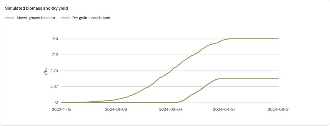
| B · WOFOST 7.2 / PCSE 6.0.13 | Moroccan Achtar timing adaptation | Homogeneous 1.2 m profile; non-infiltration fraction 0.05; no nitrogen stress |
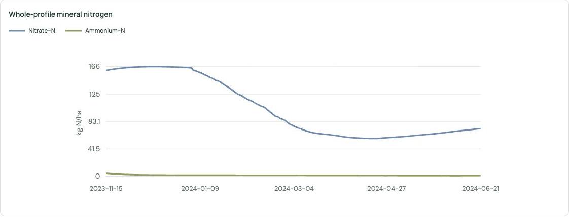
| C · APSIM Next Generation | Model default Hartog | 2 m layered profile; CN 75; nitrogen dynamics; explicit porosity cap in 3 layers |
Different stopping dates matter
| Run | Actual reported window | Rainfall / actual ET | Dry grain yield |
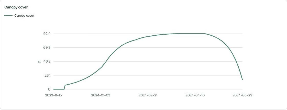
| A | 15 Nov 2023-29 May 2024; maturity | 320.7 / 388.9 mm | 10.60 t/ha |
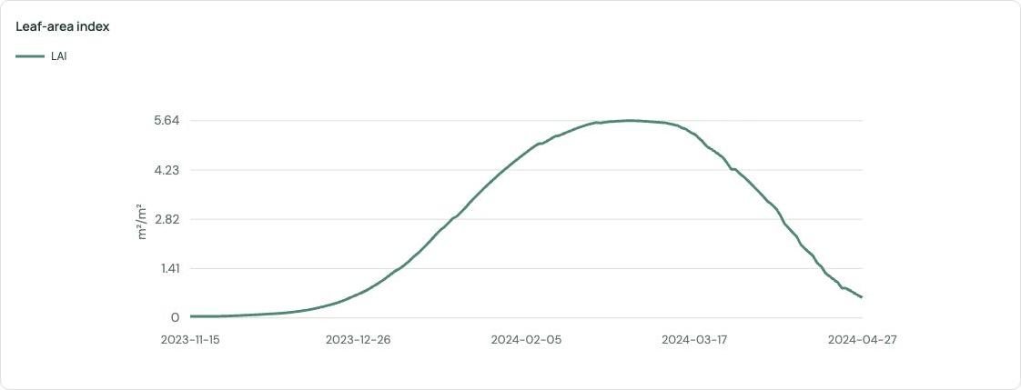
| B | 15 Nov 2023-27 Apr 2024; maturity | 301.3 / 264.7 mm | 5.83 t/ha |
| C | 15 Nov 2023-21 Jun 2024; end date, harvest ready | 336.4 / 384.0 mm | 3.51 t/ha |
These are uncalibrated scenario outputs, not observed yields. Different crop sets, stress processes, profile depths and stopping dates prevent a controlled ranking of engines. Rainfall totals differ because the reported windows differ. Whole-profile numerical water balances passed in all runs (maximum daily residual about 1e-13 mm). That establishes accounting closure only.
Capture provenance
Earlier Saïs full-page screenshots, chart crops, crop coordinates and observed result states are retained under output/pdf/figures/live. Fresh High Atlas screen captures are retained under output/pdf/figures. The AquaCrop complete run JSON is retained with the earlier comparison. These are teaching scenarios, not independent calibration or validation studies.
16A / Root-zone averages and fixed layers
Run A · AquaCrop default wheat · Saïs
16B / Storage and daily water fluxes
Run A · AquaCrop default wheat · Saïs
16C / Canopy development and dry matter
Run A · AquaCrop default wheat · Saïs
16D / WOFOST with Moroccan Achtar timing
Run B · Partial local phenology adaptation · Saïs
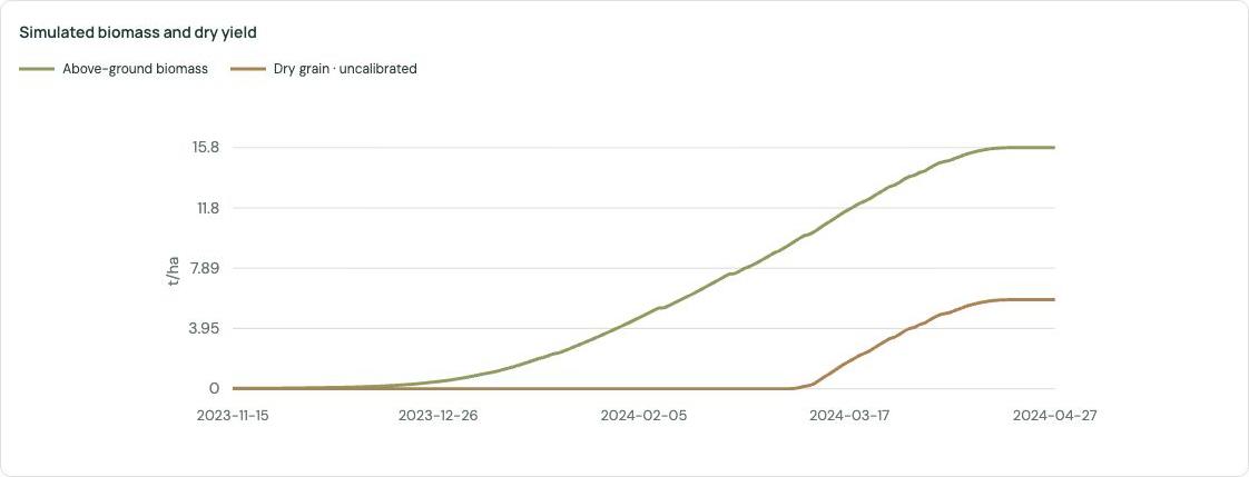
16E / APSIM nitrogen and crop growth
Run C · Hartog reference wheat · Saïs
17 / Fresh High Atlas example: WOFOST barley
Run D · Spring barley reference · High Atlas · 26 October 2026
A new live capture from the platform
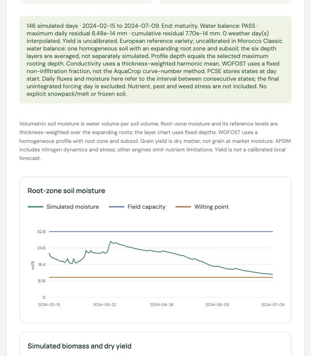
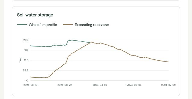
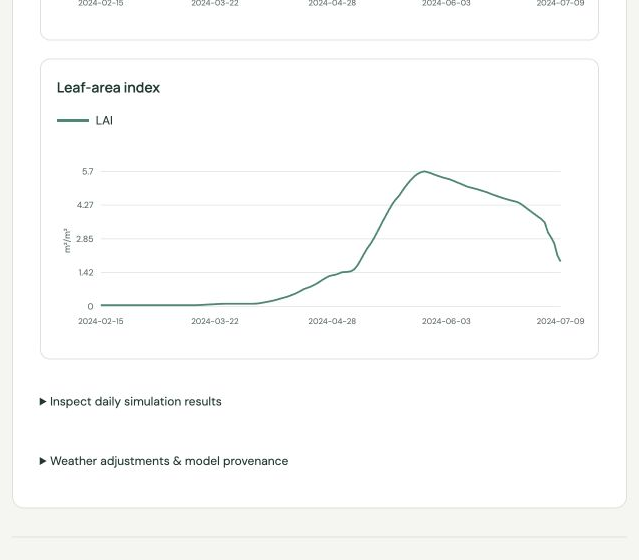
The current interface retrieved weather and soil inputs at 31.65 N, 6.43 W, elevation 1,912 m. The requested 2024 weather series contained 394 of 396 valid days; six soil horizons were available. The run used WOFOST with the European Spring_barley_301 reference crop, sowing on 15 February 2024, and simulated to maturity on 9 July 2024 (146 days). The selected maximum root depth was 1 m and initial available water was 50%. No missing weather day fell inside the simulated window.
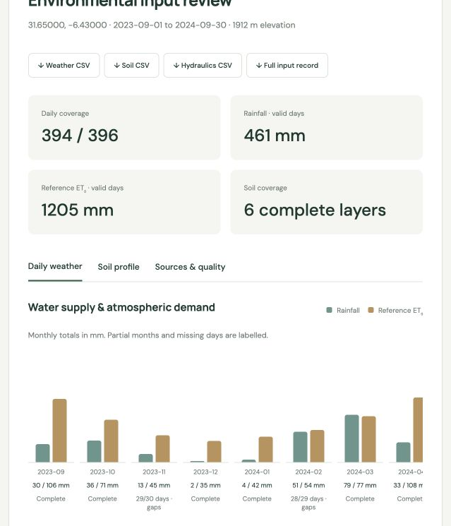 Figure 16. Weather. Retrieved rainfall and ET0 totals with day coverage. Monthly chart portion visible in this partial-window capture; ET0 is reference demand, not crop water use. | 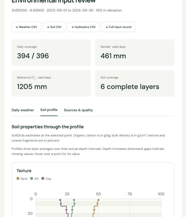 Figure 17. Soil. Profile inspection shows estimated texture by depth. Six complete horizons were available; gridded soil estimates are not field measurements. |
17 continued / Growth and water storage in the same run
Run D · WOFOST Spring_barley_301 · 15 February-9 July 2024
Important limits for this location
This example demonstrates the current workflow and graphics. The crop coefficients are not locally calibrated for High Atlas barley. The configuration does not explicitly represent snow accumulation and melt, freezing injury, vernalization requirements or terrace hydrology; coarse gridded inputs also cannot resolve field-scale elevation differences. Do not use this teaching run as a field recommendation or locally validated forecast.
18 / Comparing wheat yields across four models
A common loaded-input comparison · Saïs · 27 October 2026
The platform comparison used bread wheat at 33.8400 N, 5.6300 W, with weather loaded for 1 September 2023-31 July 2024 (334 daily weather records) and shared soil inputs. Each engine ran one season. All four rows report dry-grain yield in t/ha; the engines used their own reference crop parameters and process settings.
Figure 21. Dry-grain yields reported in the attached CropExplorer comparison view. Bars compare the displayed values only; they are not a validation score or a confidence interval.
| Engine / reference crop | Days | Actual ET (mm) | Runoff (mm) | Dry grain (t/ha) | Nitrogen scenario |
| DSSAT CERES-Wheat · Newton IB0488 | 220 | 455.14 | 1.11 | 3.739 | NO3 60 + NH4 5 kg N/ha; 100 kg N/ha calcium nitrate |
| APSIM Next Generation · Hartog | 220 | 383.97 | 3.33 | 3.508 | NO3 60 + NH4 5 kg N/ha; 100 kg N/ha nitrate |
| WOFOST 7.2 / PCSE · Winter_wheat_106 | 201 | 384.60 | 16.22 | 7.654 | Not simulated |
| AquaCrop-OSPy · Wheat | 197 | 388.91 | 21.44 | 10.596 | Not simulated |
Why the yield spread is large
The lowest and highest displayed yields differ by a factor of about 3.0 (3.508 versus 10.596 t/ha). DSSAT and APSIM are closer in this run (3.739 and 3.508 t/ha), while WOFOST is 7.654 and AquaCrop 10.596 t/ha. This is strong evidence of model-and-parameter sensitivity under one loaded scenario, not evidence that one engine is more accurate.
These runs do not isolate model structure alone
Crop parameters differ (Newton IB0488, Hartog, Winter_wheat_106 and AquaCrop Wheat). DSSAT and APSIM simulate nitrogen stress with different fertilizer forms; WOFOST and AquaCrop omit nutrients. Rooting and soil representations differ too: DSSAT’s selected depth shapes root distribution but does not cap root-tip depth. None is calibrated for this Moroccan site; DSSAT remains experimental. [3, 26, 27]
18 continued / How to interpret and follow up
Different run lengths affect water totals
DSSAT and APSIM report 220 modeled days; WOFOST reports 201 and AquaCrop 197 because maturity can end a run earlier. Thus cumulative actual ET and runoff do not all cover identical simulated periods, even though the loaded weather window is shared. The higher DSSAT actual ET total (455.14 mm) should be read alongside its run duration and engine-specific water accounting. Seasonal sums are not directly comparable as if measured over the same dates.
What the comparison does show
The four dry-grain values are useful as a structural and parameter uncertainty spread for this specified teaching scenario. The roughly threefold range warns that “same weather and soil” does not mean “same crop representation.” It is not a statistical interval, observed-yield range, or forecast bound. The two closer DSSAT/APSIM results do not independently confirm accuracy: both use explicit nitrogen scenarios and other shared settings, yet remain unvalidated reference runs.
A stronger next comparison
- Record the exact run dates, maturity/stop reason, cultivar, input record, fertilizer form/rate and rooting interpretation for each engine.
- Compare the runs over a common date window where possible. Report daily or period-normalized water use alongside totals; keep yield basis and units consistent.
- Evaluate against independent local observations for phenology, biomass, soil water, nitrogen response and grain yield. Calibrate only with suitable observations, then reserve separate seasons/sites for evaluation.
- Change one factor at a time (cultivar set, nitrogen availability, rooting, initial water or termination) to identify which assumptions explain the yield spread. Do not average the four yields as a substitute for calibration.
Run and source status
The comparison view identifies the requested location/weather selection, shared loaded soil and individual engine settings. DSSAT is now runnable for the experimental CERES-Wheat CSCER048 pathway using the Newton IB0488 reference; other DSSAT crops and active crop workbooks are not currently supported. Numerical water-balance closure and run reproducibility are useful checks, but neither establishes field-yield accuracy.
References / Models and case studies
Authoritative model documentation
The bracketed references in the background section link to the following sources. Accessed 27 October 2026. These describe model families; consult the documentation for the exact implementation and version used in an experiment.
1. FAO. AquaCrop: Calculation scheme.
https://www.fao.org/aquacrop/overview/calculation-scheme/
2. Wageningen University & Research. WOFOST: principles, production levels and implementations.
https://www.wur.nl/en/research/products-services/wofost-world-food-studies
3. DSSAT Foundation. What is DSSAT?
4. APSIM Initiative. The next generation of APSIM.
5. INRAE. General presentation of the model STICS.
https://stics.inrae.fr/eng/general-presentation-of-the-model
6. Texas A&M AgriLife / USDA. EPIC & APEX Models.
7. Akponikpè, P.B.I., Gérard, B., Michels, K. & Bielders, C. (2010). Use of the APSIM model in long term simulation to support decision making regarding nitrogen management for pearl millet in the Sahel. European Journal of Agronomy 32, 144-154. DOI: 10.1016/j.eja.2009.09.005.
https://oar.icrisat.org/6294/1/EJA_32_2_144-154_2010.pdf
Reading the guide
The background introduces concepts and selected model families. The numbered workflow chapters document CropExplorer as inspected locally. Platform-specific capabilities and restrictions take precedence over general descriptions when interpreting a CropExplorer run.
References / Moroccan parameter evidence
8. de Wit, A., Hoek, S. & Balaghi, R. (2012). Strategy report on CGMS adaptation for Morocco. E-AGRI D22.2, v2.0. Table 3, p.18; sections 1 and 2.3. Applied WOFOST wheat timing source.
https://www.e-agri.info/pdf/D22.2_Morocco_StrategyReport_F2.pdf
9. Simulation of Winter Wheat (Triticum aestivum L.) Response to Saline Irrigation Using AquaCrop in the Tadla Plain, Morocco: Implications for Irrigation Management (2026). Plants 15(12), 1899. Table 5. Partial Achtar source; omitted fields are documented in Chapter 13.
https://www.mdpi.com/2223-7747/15/12/1899
10. Hellal, F., Mansour, H., Abdel-Hady, M., El-Sayed, S. & Abdelly, C. (2019). Assessment water productivity of barley varieties under water stress by AquaCrop model. AIMS Agriculture and Food 4(3), 501-517. DOI 10.3934/agrfood.2019.3.501. Common coefficients: Table 1, p.506; variety results: Table 5.
https://www.aimspress.com/fileOther/PDF/agriculture/agrfood-04-03-501.pdf
11. Global Yield Gap Atlas. Morocco: crop-model calibration methodology. Research lead for regional barley adaptation; numeric barley parameters are not supplied in the reviewed page.
https://yieldgap-test.containers.wur.nl/Morocco
12. Mamassi et al. (2022). Relevance of soil fertility spatial databases for parameterizing APSIM-wheat crop model in Moroccan rainfed areas. Agronomy for Sustainable Development 42, 83. DOI 10.1007/s13593-022-00813-4. Table 1; APSIM Classic research reference.
https://link.springer.com/article/10.1007/s13593-022-00813-4
References / Engine and input provenance
13. AquaCrop-OSPy. Python implementation of AquaCrop-OS. App dependency: 3.1.0. The independent Python implementation is distinct from the FAO software software distribution. Generic crop sets originate in the installed library.
https://github.com/aquacropos/aquacrop
14. PCSE documentation and WOFOST crop-parameter repository. App PCSE dependency: 6.0.13; parameter branch wofost72; pinned commit fc6eda46ea0081eb0ad31fa92ea49fea60e11075.
https://pcse.readthedocs.io/en/stable/
Pinned WOFOST coefficients and metadata (wheat, barley, millet and maize); EUPL licence retained with the app.
https://github.com/ajwdewit/WOFOST_crop_parameters/tree/fc6eda46ea0081eb0ad31fa92ea49fea60e11075
15. APSIM Initiative. APSIM Next Generation documentation and official source. The platform uses the operator-installed examples and reports the runtime version in each exported run.
APSIM source and implementation reference.
https://github.com/APSIMInitiative/ApsimX
26. DSSAT CSM official engine source. CropExplorer pilot uses the CERES-Wheat module CSCER048; local pilot version 4.8.6.004.
https://github.com/DSSAT/dssat-csm-os
27. DSSAT CSM official input/data repository.
https://github.com/DSSAT/dssat-csm-data
16. Copernicus/ECMWF ERA5-Land daily aggregates, via Google Earth Engine. Weather forcing source, including documented variables and units.
https://developers.google.com/earth-engine/datasets/catalog/ECMWF_ERA5_LAND_DAILY_AGGR
17. ISRIC. SoilGrids: global gridded soil information. Soil properties at six standard depth intervals; estimates rather than local field measurements.
https://isric.org/explore/soilgrids
References / Methods, data and further work
18. Simons, G., Koster, R. & Droogers, P. (2020). HiHydroSoil v2.0: High resolution soil maps of global hydraulic properties. FutureWater Report 213. Hydraulic limits and conductivity estimates.
https://www.futurewater.nl/solutions/hihydrosoil/
19. GEE Community Catalog. HiHydroSoil v2.0 dataset access and collection details used by the app.
https://gee-community-catalog.org/projects/hihydro_soil/
20. KALRO. Maize agronomy. Kenyan context for the Katumani teaching case; not a source of fitted engine coefficients in this app.
https://www.kalro.org/maize/maize-agronomy/
21. Devkota et al. (2022). Conservation agriculture improves agronomic, economic, and soil fertility indicators for a clay soil in a rainfed Mediterranean climate in Morocco. Agricultural Systems. DOI 10.1016/j.agsy.2022.103470. Research lead; no direct APSIM parameter transfer.
https://doi.org/10.1016/j.agsy.2022.103470
22. Asseng et al. (2013). Uncertainty in simulating wheat yields under climate change. Nature Climate Change 3, 827-832. Methodological reference for future intercomparison.
https://doi.org/10.1038/nclimate1916
23. Asseng et al. (2015). Rising temperatures reduce global wheat production. Nature Climate Change 5, 143-147. Further intercomparison reading.
https://doi.org/10.1038/nclimate2470
24. Allen, R.G., Pereira, L.S., Raes, D. & Smith, M. (1998). Crop evapotranspiration: Guidelines for computing crop water requirements. FAO Irrigation and Drainage Paper 56. Reference ET0 method.
https://www.fao.org/4/x0490e/x0490e00.htm
25. NASA/USGS. SRTM GL1 30 m, via Earth Engine. Elevation input for reference calculations.
https://developers.google.com/earth-engine/datasets/catalog/USGS_SRTMGL1_003
CropExplorer · Crop Modeling Platform · Center for Applied Systems Analysis, CAES, UM6P